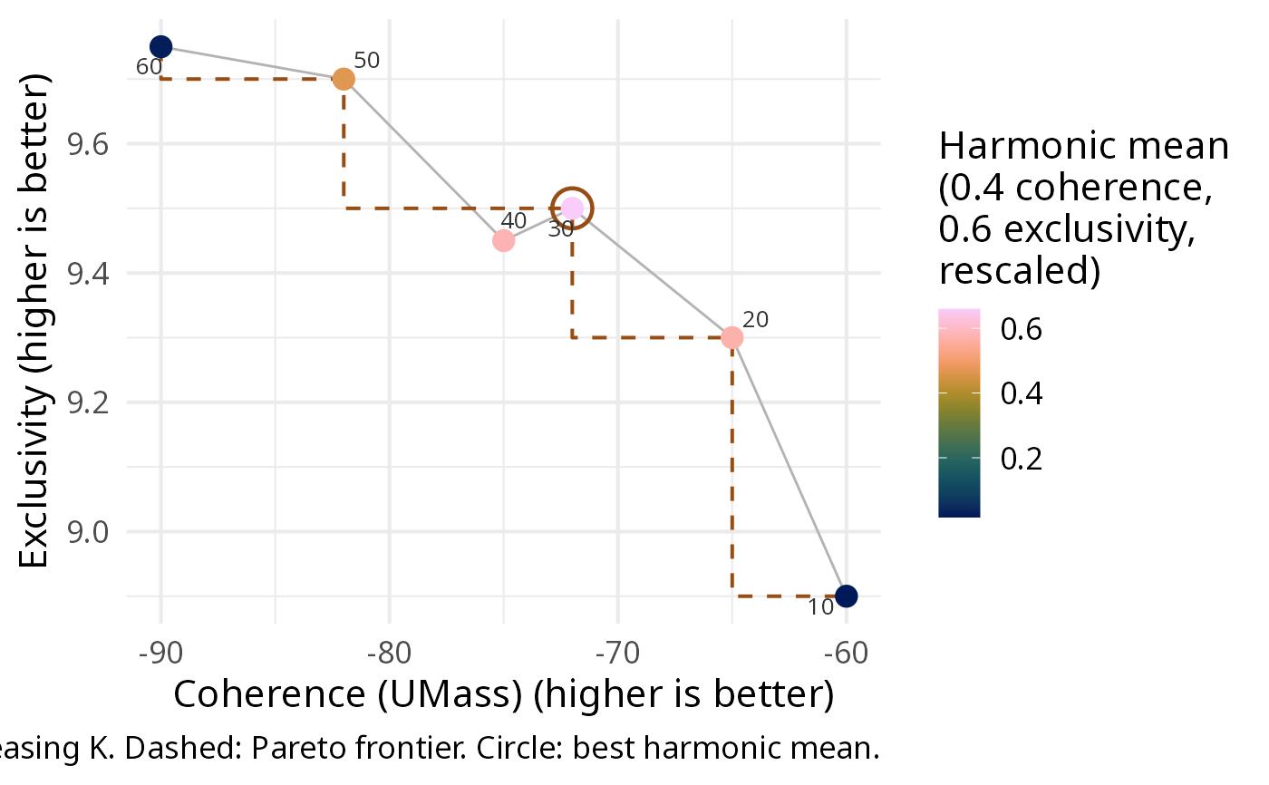
Coherence-exclusivity frontier of a grid of topic models

Place each model in the coherence x exclusivity plane, join the models in order of K, draw the Pareto frontier (pareto_frontier(): only these models are worth considering), colour the points by the weighted harmonic mean of the two criteria (coherence_exclusivity_score()) and circle the best model. With several corpora (vocabulary filters), one panel per corpus.

Coherence favours few broad topics and exclusivity many narrow ones, so no K maximises both (Roberts et al. 2014): the frontier shows the trade-off, the weights say how much each criterion matters to you.

Usage

plot_k_frontier(
  x,
  coherence = "coherence_umass",
  exclusivity = "exclusivity",
  k = "K",
  by = NULL,
  weights = c(0.4, 0.6),
  rescale = TRUE,
  base_size = 16,
  palette = "batlow",
  ...
)

Arguments

x: A topic_model_evaluation (evaluate_topic_models()), or a table with one row per model (e.g. stm::searchK()$results). Runs are averaged.
coherence, exclusivity, k: Column names of the coherence, the exclusivity and the number of topics.
by: Column name(s) of the grouping (one panel each). Default: "corpus" when there are several corpora.
weights, rescale: Passed to coherence_exclusivity_score().
base_size: Numeric scalar, base font size of the theme.
palette: A continuous scico palette for the score.
...: Not used: an argument renamed in the development version of mintR gives an error naming its replacement.

Value

A ggplot. Its data (plot$data) is the model table with score and pareto added.

References

Roberts, M. E., Stewart, B. M., Tingley, D., Lucas, C., Leder-Luis, J., Gadarian, S. K., Albertson, B. and Rand, D. G. (2014). Structural topic models for open-ended survey responses. American Journal of Political Science, 58(4), 1064-1082. doi:10.1111/ajps.12103

Examples

results <- data.frame(
  K = seq(10, 60, 10),
  coherence_umass = c(-60, -65, -72, -75, -82, -90),
  exclusivity = c(8.9, 9.3, 9.5, 9.45, 9.7, 9.75)
)
plot_k_frontier(results)